vizChord

Visualizing brain connectivity profiles with a chord diagram

vizChord(
  data,
  hot = "#F8766D",
  cold = "#00BFC4",
  width = 1200,
  height = 1200,
  filename = "conn.png",
  colorscheme,
  title,
  leg.height = 100,
  ncol = 1,
  nrow = 1,
  colorbar_title = "Connectivity Strength"
)

Arguments

data

a vector of edge values with a length of 78, 4005, 7021, 23871 or 30135.

hot

color for the positive connections.Set to #F8766D by default.

cold

color for the negative connections.Set to #00BFC4 by default.

width

width (in pixels) of each connectogram. Set to 1200 by default.

height

height (in pixels) of each connectogram . Set to 1200 by default.

filename

output filename with a *.png file extension. Set to conn.png by default

colorscheme

an optional vector of color names or color codes to color code the networks.

title

a vector of strings to be used as title

leg.height

height (in pixels) of legend, in pixels. Set to 100 by default. Not used for single row data

ncol

number of columns in the plot. Not used for single row data

nrow

number of rows in the plot. Not used for single row data

colorbar_title

title for the colorbar legend

Value

outputs a .png image

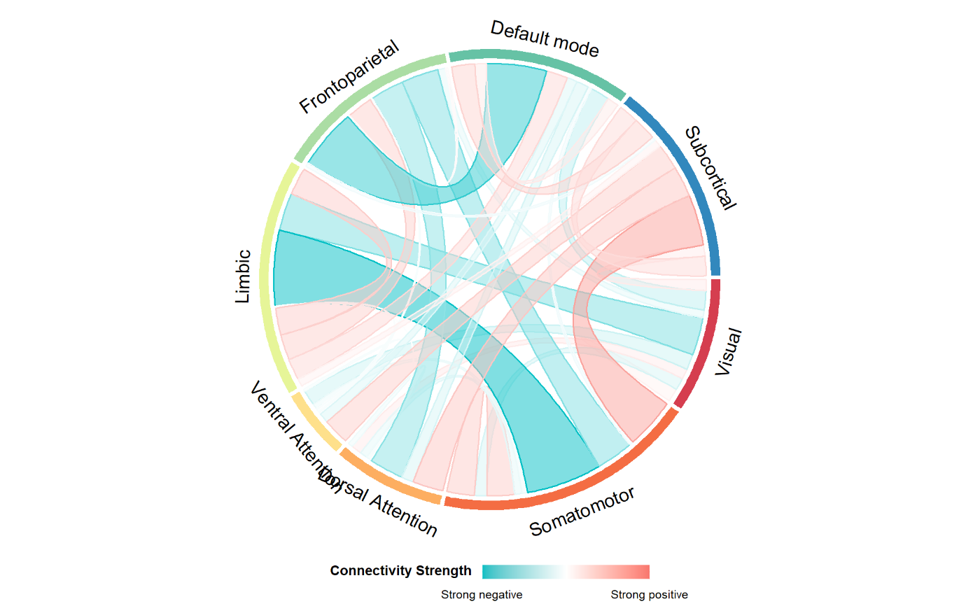
Details

This function takes a matrix (NROW=number of edges in the connectome; NCOL=number of edges in the connectome) of edge values and visualizes the average network-to-network connectivity in a chord diagram.

Examples

results=runif(7021, min = -1, max = 1)
vizChord(data=results, filename="FC_chord119.png")