Example analyses with VertexWiseR - Example 2
Charly Billaud, Junhong Yu
2025-07-16
VertexWiseR_Example_2.RmdExample 2: Mixed effect model of intervention-related changes on hippocampal thickness
Note: This is the most up-to-date demo. Its version published in Imaging Neuroscience (2024) 2: 1–14 no longer applies since the v1.3.0 fixes made to the TFCE_vertex_analysis_mixed() function (see our updates page for details).
The analysis will use surface data already extracted in R from a preprocessed subjects directory, which we make available so you do not need to preprocess a sample yourself. To obtain it, we had extracted thickness data from a Hippunfold preprocessing directory of the Fink dataset (Fink et al. 2021).
The demo data (~216 MB) required to run the example analysis, and can be downloaded from the package’s github repository with the following function:
#This will save the demo_data directory in a temporary directory (tempdir(), but you can change it to your own path)
demodata=VertexWiseR:::dl_demo(path=tempdir(), quiet=TRUE)
Here is the command line which was originally used to extract the surface:
#HIPvextract(sdirpath = hippunfold_SUBJECTS_DIR, filename = "FINK_Tv", measure = "thickness", subj_ID = T)To load the hippocampal thickness matrix:
To smooth the surface data:
FINK_Tv_smoothed_ses13 = smooth_surf(FINK_Tv_ses13, 5)To load the behavioural data (FINK_behdata_ses13.csv, which contains two rows per participant, for scanning sessions 1 and 3).
Here, we are interested in the interaction between session number (time) and group. To run the vertex-wise mixed model analysis with random field theory-based cluster correction, testing for the effect of session, group, session * group interaction, on hippocampal thickness, with subject ID as a random variable:
model2_RFT=RFT_vertex_analysis(
  model = dat_beh_ses13[,c("session","group","session_x_group")],
  contrast = dat_beh_ses13[,"session_x_group"],
  surf_data=FINK_Tv_smoothed_ses13,
  random=dat_beh_ses13[,"participant_id"], p=0.05)
model2_RFT$cluster_level_results## $`Positive contrast`
## clusid nverts P X Y Z tstat region
## 1 1 974 0.041 -13.3 27.5 1.3 4.14 L Subiculum
##
## $`Negative contrast`
## [1] "No significant clusters"To run the vertex-wise mixed model analysis with threshold-free cluster enhancement-based cluster correction, with 1000 permutations, testing for the effect of session, group, session * group interaction, on hippocampal thickness, with subject ID as a random variable:
set.seed(123)
model2_TFCE=TFCE_vertex_analysis_mixed(
  model = dat_beh_ses13[,c("session","group","session_x_group")],
  contrast = dat_beh_ses13[,"session_x_group"],
  surf_data= FINK_Tv_smoothed_ses13,
  nperm=1000,
  random = dat_beh_ses13[,"participant_id"],
  perm_type="within_between",
  nthread=4)
TFCEoutput = TFCE_threshold(model2_TFCE, p=0.05)
TFCEoutput$cluster_level_results## $`Positive contrast`
## clusid nverts P X Y Z tstat region
## 1 1 73 0.033 -13.3 27.5 1.3 4.14 L Subiculum
##
## $`Negative contrasts`
## [1] "No significant clusters"To plot the significant clusters from both models on the CITI168 hippocampal template surface:
tmaps = rbind(model2_RFT$thresholded_tstat_map, TFCEoutput$thresholded_tstat_map)
plot_surf(surf_data = tmaps,
          filename = 'FINK_tstatmaps.png',
          title=c('RFT-corrected\nclusters','TFCE-corrected\nclusters'),
          cmap='Reds',
          show.plot.window=TRUE)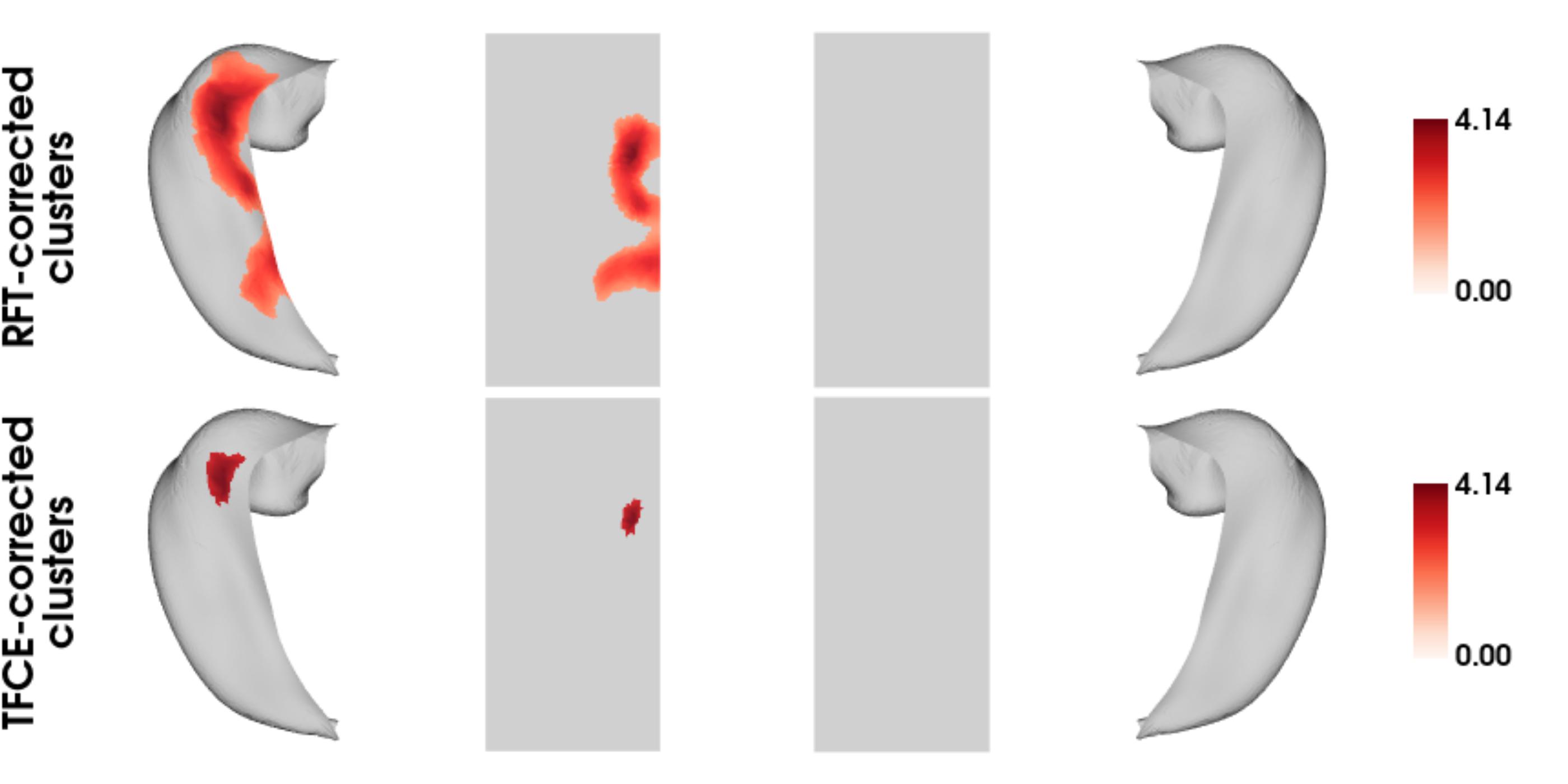
Example 2 follow-up: plotting and post-hoc analyses of hippocampal clusters across regression models
The code below was used in R (v.4.3.3) to plot the cluster-wise values from the RFT and TFCE corrected analyses and validate them with additional mixed linear models.
We produce a figure displaying the thickness of the hippocampal clusters in relation to the group and session variables, in RFT and TFCE models, demonstrating a steeper curve toward group 2:
#We divide the cluster values by their sum to get the average thickness per vertex
dat_beh_ses13$clustCTTFCE=(FINK_Tv_smoothed_ses13 %*% TFCEoutput$pos_mask)/sum(TFCEoutput$pos_mask>0)
dat_beh_ses13$clustRFT=(FINK_Tv_smoothed_ses13 %*% model2_RFT$pos_mask)/sum(model2_RFT$pos_mask>0)

library(ggplot2)
library(ggbeeswarm)
library(cowplot)

a=ggplot(data=dat_beh_ses13,aes(y=clustCTTFCE,x=as.factor(session), color=as.factor(group)))+
  geom_quasirandom(dodge.width=0.5)+
  geom_line(aes(group=participant_id), alpha=0.2)+
  geom_smooth(aes(group=group), method="lm")+
  labs(y="Mean thickness (mm)", x="session", color="group")+
  guides(colour = "none")+
  ggtitle("Positive cluster\n (TFCE-corrected)")+
  ylim(1.1, 1.55)

b=ggplot(data=dat_beh_ses13,aes(y=clustRFT,x=as.factor(session), color=as.factor(group)))+
  geom_quasirandom(dodge.width=0.5)+
  geom_line(aes(group=participant_id), alpha=0.2)+
  geom_smooth(aes(group=group), method="lm")+
  labs(y="Mean thickness (mm)", x="session", color="group")+
  ggtitle("Positive cluster\n(RFT-corrected)")+
  scale_color_discrete(name="Group",labels=c("group 1", "group 2"))+
  ylim(1.1, 1.55)

#to write the image file
#png(filename="traj.png", res=250, width=1400,height=604)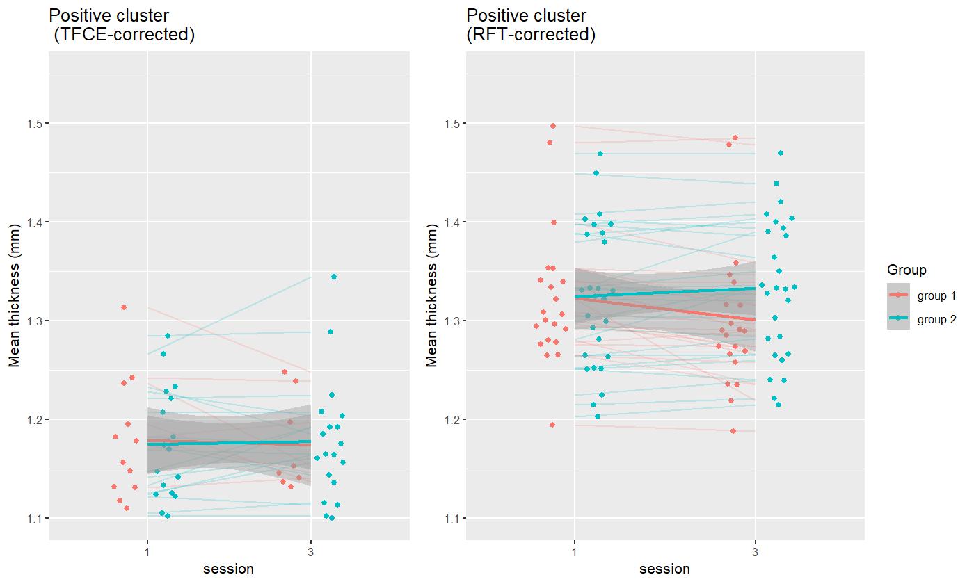
## null device
##           1
As an additional validation of these results, these significant clusters were extracted as regions-of-interests and fitted in a linear mixed effects model using another R package— lmerTest (Kuznetsova, Brockhoff, and Christensen 2017).
Linear mixed effect testing the effect of session, group, and session * group interaction on the positive RFT clusters’ average thickness value
lme.RFT=lmer(clustRFT~session+group+session*group+(1|participant_id),data =dat_beh_ses13 )
summary(lme.RFT)
## Linear mixed model fit by REML. t-tests use Satterthwaite's method [
## lmerModLmerTest]
## Formula: clustRFT ~ session + group + session * group + (1 | participant_id)
## Data: dat_beh_ses13
##
## REML criterion at convergence: -317.1
##
## Scaled residuals:
## Min 1Q Median 3Q Max
## -2.69862 -0.43221 -0.04002 0.42291 2.57082
##
## Random effects:
## Groups Name Variance Std.Dev.
## participant_id (Intercept) 0.004837 0.06955
## Residual 0.000236 0.01536
## Number of obs: 96, groups: participant_id, 48
##
## Fixed effects:
## Estimate Std. Error df t value Pr(>|t|)
## (Intercept) 1.326760 0.010717 54.685962 123.801 < 2e-16 ***
## session -0.003450 0.001580 46.000000 -2.183 0.0342 *
## group -0.006877 0.010717 54.685962 -0.642 0.5237
## session:group 0.007645 0.001580 46.000000 4.837 1.51e-05 ***
## ---
## Signif. codes: 0 '***' 0.001 '**' 0.01 '*' 0.05 '.' 0.1 ' ' 1
##
## Correlation of Fixed Effects:
## (Intr) sessin group
## session -0.295
## group -0.125 0.037
## session:grp 0.037 -0.125 -0.295Linear mixed effect testing the effect of session, group, and session * group interaction on the positive TFCE clusters’ average thickness value
lme.posTFCE=lmer(clustCTTFCE~session+group+session*group+(1|participant_id),data =dat_beh_ses13 )
summary(lme.posTFCE)
## Linear mixed model fit by REML. t-tests use Satterthwaite's method [
## lmerModLmerTest]
## Formula: clustCTTFCE ~ session + group + session * group + (1 | participant_id)
## Data: dat_beh_ses13
##
## REML criterion at convergence: -272.9
##
## Scaled residuals:
## Min 1Q Median 3Q Max
## -1.50112 -0.45415 -0.05631 0.49916 1.71410
##
## Random effects:
## Groups Name Variance Std.Dev.
## participant_id (Intercept) 0.0048047 0.06932
## Residual 0.0005989 0.02447
## Number of obs: 96, groups: participant_id, 48
##
## Fixed effects:
## Estimate Std. Error df t value Pr(>|t|)
## (Intercept) 1.134943 0.011549 66.462361 98.275 < 2e-16 ***
## session -0.003589 0.002517 46.000000 -1.426 0.160692
## group -0.009920 0.011549 66.462361 -0.859 0.393452
## session:group 0.010234 0.002517 46.000000 4.065 0.000186 ***
## ---
## Signif. codes: 0 '***' 0.001 '**' 0.01 '*' 0.05 '.' 0.1 ' ' 1
##
## Correlation of Fixed Effects:
## (Intr) sessin group
## session -0.436
## group -0.125 0.054
## session:grp 0.054 -0.125 -0.436